Tutorial¶

For an explanation of the algorithm and motivation behind leabra7, see Prof. Randy O’Reilly’s book Computational Cognitive Neuroscience. This tutorial assumes general familiarity with the concepts in that book, and focuses on the mechanics of using the leabra7 package.

Contents:

Two neurons
Pattern association

Two neurons ¶

The simplest leabra7 network consists of two neurons, with one neuron driving the other. First, import the necessary libraries:

import matplotlib.pyplot as plt
import pandas as pd
import leabra7 as lb

from typing import *

Now, we can create an empty network:

net = lb.Net()

We can now add two layers, each with one neuron:

layer_spec = lb.LayerSpec(
    log_on_cycle=("unit_v_m",
                  "unit_act",
                  "unit_i_net",
                  "unit_net",
                  "unit_gc_i",
                  "unit_adapt",
                  "unit_spike"))
net.new_layer(name="input", size=1, spec=layer_spec)
net.new_layer(name="output", size=1, spec=layer_spec)

Each layer gets a spec (“specification”) object which contains simulation parameters. In this case, the log_on_cycle parameter tells the network to record each of the following attributes every cycle:

"unit_v_m: The membrane potential of each neuron
"unit_act": The activation of each neuron
"unit_i_net": The net current into each neuron
"unit_net": The net input into each neuron
"unit_gc_i": The inhibitory current in each neuron
"unit_adapt": The adaption current in each neuron
"unit_spike": Whether the neuron is spiking

Spec objects can be used to specify many more parameters; see Spec Objects for more information.

Connect the two layers with a projection:

net.new_projn(name="proj1", pre="input", post="output")

Before cycling the network, we will force the input layer to have an activation of 1:

net.clamp_layer(name="input", acts=[1])

The acts parameter is the sequence of activations that the input layer will be clamped to. It does not have to specify a value for every unit, since shorter patterns will be tiled.

Now, we can cycle the network:

for _ in range(200):
    net.cycle()

Let’s retrieve the network logs:

wholeLog, partLog = net.logs(freq="cycle", name="output")

The returned logs are simply Pandas dataframes.

Note that there are two kinds of logs: whole logs, and part logs. Whole logs contain attributes that pertain to the whole object, for example, the average activation of a layer. Part logs contain attributes that pertain to the parts of an object. Since units are parts of a layer, and we logged entirely unit attributes, we will work with the parts logs:

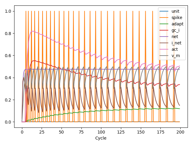
We can plot the Pandas dataframe:

partLog = partLog.drop(columns=["unit"])
ax = partLog.plot(x="time")
ax.set_xlabel("Cycle")

Pattern association ¶

Now, we will try a slightly more complicated task: training a network to recognize a simple set of patterns. First, as usual, we will import the necessary libraries. We will also configure a project name and set up Python’s logging library to timestamp all of our logs (this is useful for tracking the progress of training):

import logging
import sys
from typing import *
import numpy as np
import pandas as pd

import leabra7 as lb

PROJ_NAME = "pat_assoc"

logging.basicConfig(
    level=logging.DEBUG,
    format="%(asctime)s %(levelname)s %(message)s",
    handlers=(logging.FileHandler(
        "{0}_log.txt".format(PROJ_NAME), mode="w"),
              logging.StreamHandler(sys.stdout)))

With this housekeeping out of the way, we can start to write the actual network training code. We will break down the task of training a network into a series of functions that can be modified for any general network training task. First, define a function to load and preprocess the input and output data:

def load_data() -> Tuple[np.ndarray, np.ndarray]:
    """Loads and preprocesses the data.

    Returns:
      An (X, Y) tuple containing the features and labels,
      respectively.

    """
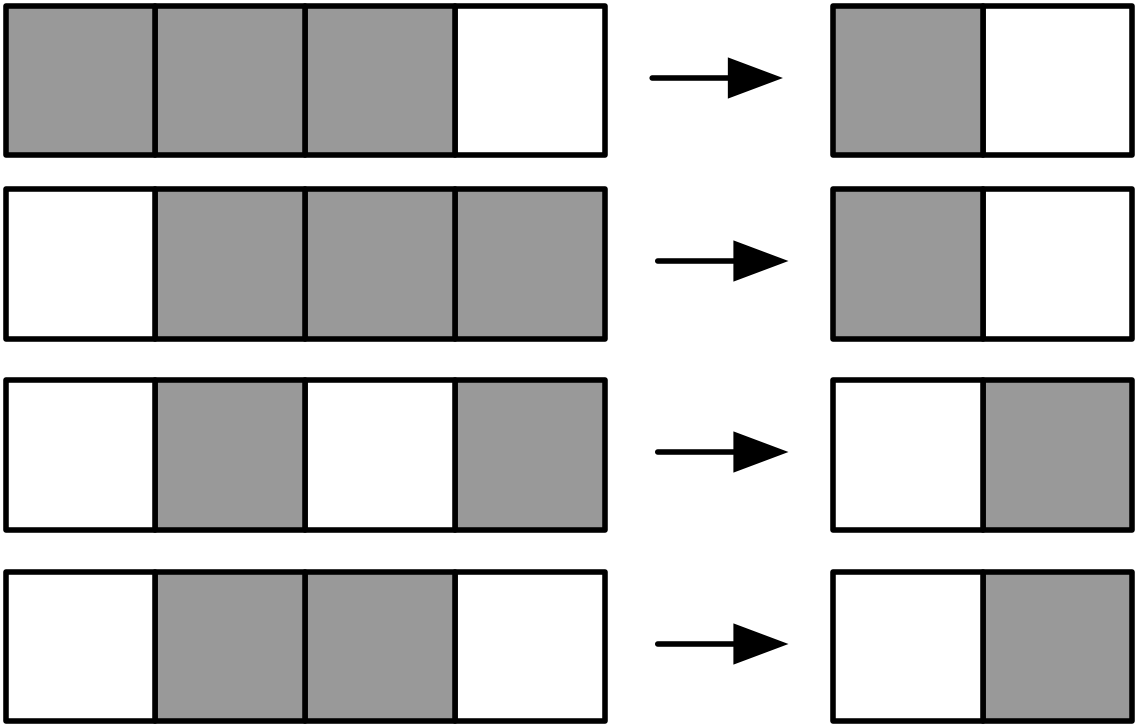
    X = np.array([
        [1, 1, 1, 0],
        [0, 1, 1, 1],
        [0, 1, 0, 1],
        [0, 1, 0],
    ])
    Y = np.array([
        [1, 0],
        [1, 0],
        [0, 1],
        [0, 1]
    ])
    return (X, Y)

In this case, we are loading the following pattern associations:

We follow scikit-learn’s convention of using the array shape [n_samples, n_features].

Now, we will define a function to construct the network. We will use a simple feedforward architecture with one input layer and one output layer.

def build_network() -> lb.Net:
    """Builds the classifier network.

    Returns:
      A leabra7 network for classification.

    """
    logging.info("Building network")
    net = lb.Net()

    # Layers
    layer_spec = lb.LayerSpec(
        gi=1.5,
        ff=1,
        fb=0.5,
        fb_dt=0.7,
        unit_spec=lb.UnitSpec(
            adapt_dt=0,
            vm_gain=0,
            spike_gain=0,
            ss_dt=1,
            s_dt=0.2,
            m_dt=0.15,
            l_dn_dt=0.4,
            l_up_inc=0.15,
            vm_dt=0.3,
            net_dt=0.7))
    net.new_layer("input", size=4, spec=layer_spec)
    net.new_layer("output", size=2, spec=layer_spec)

    # Projections
    spec = lb.ProjnSpec(
        lrate=0.02,
        dist=lb.Uniform(0.25, 0.75),
        thr_l_mix=0.01,
        cos_diff_lrate=False)
    net.new_projn("input_to_output", pre="input", post="output", spec=spec)

    return net

In this case, we have tweaked many of the parameters. This is not strictly necessary, but it helps this specific network train faster.

Now, we will define a function to run a network trial, consisting of a minus and a plus phase. In the minus phase, the input pattern will be clamped to the network’s input layer, and the network will be cycled. In the plus phase, both the input and the output patterns will be clamped to their respective layers, and the network will be again cycled. The difference between these two phases (actual and expectation) will drive learning.

def trial(network: lb.Net, input_pattern: Iterable[float],
          output_pattern: Iterable[float]) -> None:
    """Runs a trial.

    Args:
      input_pattern: The pattern to clamp to the network's input layer.
      output_pattern: The pattern to clamp to the network's output layer.

    """
    network.clamp_layer("input", input_pattern)
    network.minus_phase_cycle(num_cycles=50)
    network.clamp_layer("output", output_pattern)
    network.plus_phase_cycle(num_cycles=25)
    network.unclamp_layer("input")
    network.unclamp_layer("output")
    network.learn()

The next function we will define will run an epoch, where one trial is run for each pattern in the dataset:

def epoch(network: lb.Net, input_patterns: np.ndarray,
          output_patterns: np.ndarray) -> None:
    """Runs an epoch (one pass through the whole dataset).

    Args:
      input_patterns: A numpy array with shape (n_samples, n_features).
      output_patterns: A numpy array with shape (n_samples, n_features).

    """
    for x, y in zip(input_patterns, output_patterns):
        trial(network, x, y)
    network.end_epoch()

With these building blocks in place, we can write the main training function:

def train(network: lb.Net,
          input_patterns: np.ndarray,
          output_patterns: np.ndarray,
          num_epochs: int = 3000) -> pd.DataFrame:
    """Trains the network.

    Args:
      input_patterns: A numpy array with shape (n_samples, n_features).
      output_patterns: A numpy array with shape (n_samples, n_features).
      num_patterns: The number of epochs to run. Defaults to 500.

    Returns:
      pd.DataFrame:  A dataframe of metrics from the training run.

    """
    logging.info("Begin training")

    data: Dict[str, List[float]] = {
        "epoch": [],
        "train_loss": [],
    }

    perfect_epochs = 0
    for i in range(num_epochs):
        epoch(network, input_patterns, output_patterns)
        pred = predict(network, input_patterns)
        data["epoch"].append(i)
        data["train_loss"].append(mse_thresh(output_patterns, pred))

        logging.info("Epoch %d/%d. Train loss: %.4f", i, num_epochs,
                      data["train_loss"][-1])

        if data["train_loss"][-1] == 0:
            perfect_epochs += 1
        else:
            perfect_epochs = 0

        if perfect_epochs == 3:
            logging.info("Ending training after %d perfect epochs.",
                          perfect_epochs)
            break

    return pd.DataFrame(data)

This training function continuously runs epochs until we get three perfect epochs in a row, or we hit 3000 epochs. It also records the training loss for each epoch, and returns the recorded metrics at the end of training.

The training function makes use of two housekeeping functions which we will now define:

The thresholded mean-squared-error loss function, which measures the performance of the network.
The prediction function, which calculates predictions for an array of input patterns.

First, let’s define the thresholded MSE loss function:

def mse_thresh(expected: np.ndarray, actual: np.ndarray) -> float:
    """Calculates the thresholded mean squared error.

    If the error is < 0.5, it is treated as 0 (i.e., we count < 0.5 as 0 and
    > 0.5 as 1).

    Args:
      expected: The expected output patterns, with shape [n_samples, n_features].
      actual: The actual output patterns, with shape [n_samples, n_features].

    Returns:
      The thresholded mean square error.

    """
    diff = np.abs(expected - actual)
    diff[diff < 0.5] = 0
    return np.mean(diff * diff)

And now, the prediction function:

def output(network: lb.Net, pattern: Iterable[float]) -> List[float]:
    """Calculates a prediction for a single input pattern.

    Args:
      network: The trained network.
      pattern: The input pattern.

    Returns:
      np.ndarray: The output of the network after clamping the input
      pattern to the input layer and settling. The max value is set to one,
      everything else is set to zero.

    """
    network.clamp_layer("input", pattern)
    for _ in range(50):
        network.cycle()
    network.unclamp_layer("input")
    out = network.observe("output", "unit_act")["act"].values
    return list(out)


def predict(network: lb.Net, input_patterns: np.ndarray) -> np.ndarray:
    """Calculates predictions for an array of input patterns.

    Args:
        network: The trained network.
        input_patterns: An array of shape (n_samples, n_features)
            containing the input patterns for which to calculate predictions.

    Returns:
        np.ndarray: An array of shape (n_samples, n_features) containing the
            predictions for the input patterns.

    """
    outputs = []
    for item in input_patterns:
        outputs.append(output(network, item))
    return np.array(outputs)

That was a lot of work, but we can now train the network with a few lines of code!

X, Y = load_data()
net = build_network()
metrics = train(net, X, Y)

# Save metrics and network for future analysis
metrics.to_csv("{0}_metrics.csv".format(PROJ_NAME), index=False)
net.save("{0}_network.pkl".format(PROJ_NAME))

The script’s output should look something like this:

2018-09-06 22:07:50,202 INFO Begin training pat_assoc
2018-09-06 22:07:50,202 INFO Building network
2018-09-06 22:07:50,204 INFO Begin training
2018-09-06 22:07:50,460 INFO Epoch 0/3000. Train loss: 0.6138
2018-09-06 22:07:50,709 INFO Epoch 1/3000. Train loss: 0.5818
2018-09-06 22:07:50,963 INFO Epoch 2/3000. Train loss: 0.5814
2018-09-06 22:07:51,215 INFO Epoch 3/3000. Train loss: 0.5811

...

2018-09-06 22:09:27,980 INFO Epoch 392/3000. Train loss: 0.0319
2018-09-06 22:09:28,227 INFO Epoch 393/3000. Train loss: 0.0315
2018-09-06 22:09:28,476 INFO Epoch 394/3000. Train loss: 0.0000
2018-09-06 22:09:28,722 INFO Epoch 395/3000. Train loss: 0.0000
2018-09-06 22:09:28,970 INFO Epoch 396/3000. Train loss: 0.0000
2018-09-06 22:09:28,971 INFO Ending training after 3 perfect epochs.

At which point the network will have learned to perfectly recognize the desired patterns. That is to say, when we clamp the input pattern to the input layer and cycle the network, the correct output pattern will be reproduced on the out layer.

The file pat_assoc_metrics.csv can be further analyzed as you like, and the network can be easily loaded from the pat_assoc_network.pkl file in the future. See the network reference for more information.

Tutorial¶

Two neurons ¶

Pattern association ¶

leabra7

Navigation

Related Topics

Tutorial¶

Two neurons¶

Pattern association¶

Two neurons ¶

Pattern association ¶